Outage probability

In this post, we will look at the techniques used to obtain the success probability of a typical source-destination pair in a Poisson network. We will look at common fading models like Rayleigh, Nakagami-m and ${\chi^2}$ distributions, and obtain the success probability in the ${\mathtt{SINR}}$ model.

1. System Model

The transmitters are modeled as a stationary and isotropic Poisson point process ${\Phi}$ on the plane ${{\mathbb R}^2}$ . The fading between two nodes ${x}$ and ${y}$ is denoted by ${\mathtt{h}_{xy}}$ and is assumed i.i.d. between any pair of nodes. The path loss function denoted by ${\ell(x)}$ and is given by ${\ell(x)=\|x\|^{-\alpha}}$ . The interference at location ${y}$ is given by

$\displaystyle \mathtt{I}(y)=\sum_{x \in \Phi} \mathtt{h}_{xy} \ell(x-y).$

Each node is associated with a virtual receiver at a distance ${R}$ in a random direction. These receivers are not part of the point process ${\Phi}$ . This model is often referred to as the dumbbell model in the literature [Baccelli]. The signal-to-interference and noise ratio between nodes ${x}$ and its receiver ${y}$ denoted by ${\mathtt{SINR}(x,y)}$ is defined as

$\displaystyle \mathtt{SINR}(x,y)=\frac{\mathtt{h}_{xy}\ell(x-y)}{\sigma^2+I(y)} .$

1.1. Typical transmitter

What exactly do we mean by the outage probability of a link in a Poisson network? Since we are considering a homogeneous point process, all the nodes are same, and we can pick any node in random and observe the outage probability. But what exactly do we mean by picking a node? This leads to the concept of conditional probability on point process, a.k.a the Palm probabilities. So we essentially condition on the fact that a point of the process is located at the origin and find the outage probability for its link. More precisely,

where ${\mathbb{P}^{!o}}$ is the reduced Palm measure [Stoyan]. The reduced Palm probability should be interpreted as conditioning a point of the point process ${\Phi}$ to be at the origin, but not counting it towards the computation of interference. So to compute the success probability, we should know the reduced Palm measure of the underlying point process. A nice example to illustrate the concept of the reduced Palm measure is the nearest neighbor distance (NN) distribution. The NN distribution is

$\displaystyle \mathop{\mathbb P}(NN> r) = \mathbb{P}^{!o}(\Phi( B(o,r)) = 0),$

where ${\Phi(B(o,r))}$ is the number of points of ${\Phi}$ in the ball of radius ${r}$ . So in this example, we condition on there being a point at the origin but do not count it (the reduced Palm measure).

The reduced Palm measure for a PPP is characterized by Slyvniak’s theorem [Stoyan].

Theorem 1(Slyvniak) For a Poisson point process $\displaystyle \mathbb{P}^{!x}=\mathop{\mathbb P}.$

What this theorem says is, for a Poisson point process the reduced Palm measure is equal to the original measure. So in a PPP, we can add a point at any location without changing the properties of the underlying node distribution (of course the added point should not be considered). The remarkable Palm characterization of the PPP follows from its independence properties, and it turns out that Slyvniak’s theorem is a characterization of the PPP.

Observe that such simple characterization does not hold true for all non-stationary PPP. For example consider a two dimensional lattice ${{\mathbb Z}^2+U([0,1]^2]}$ , where ${U}$ denotes uniform noise. If we condition an there being a node at the origin, then we can immediately observe that there should be some points at locations given by ${{\mathbb Z}^2}$ .

2. Success Probability

In this section we look at the success probability of a typical link when the fading distributions are of the exponential form. We begin with the simplest case when ${\mathtt{h}_{}}$ is exponentially distributed. This is the case when the fading (amplitude) is Rayliegh distributed, and hence its power is exponentially distributed. This is a very common distribution of fading used in the wireless literature and occurs when there is sufficient scattering.

2.1. Rayleigh fading: ${ \mathtt{h}_{}\sim \exp(1)}$

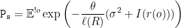
The success probability from (1) is

$\displaystyle \mathtt{P_s} =\mathbb{P}^{!o}\left(\frac{\mathtt{h}_{o}\ell(R)}{\sigma^2+\mathtt{I}(r(o))} \geq \theta\right)$

Since ${\mathtt{h}_{}}$ is exponentially distributed,

$\displaystyle \mathtt{P_s}=\mathbb{E}^{!o}\exp\left(-\frac{\theta}{\ell(R)}(\sigma^2+I(r(o))) \right)$

$\displaystyle \begin{array}{rcl} \mathtt{P_s}&=&\exp\left(-\frac{\theta}{\ell(R)}\sigma^2\right)\mathbb{E}^{!o}\exp\left(- \frac{\theta}{\ell(R)}I(r(o)) \right)\\ &\stackrel{(a)}{=}&\exp\left(-\frac{\theta}{\ell(R)}\sigma^2\right)\mathbb{E}^{!o}\exp\left(- \frac{\theta}{\ell(R)}I(r(o)) \right)\\ &\stackrel{(b)}{=}&\exp\left(-\frac{\theta}{\ell(R)}\sigma^2\right)\mathbb{E}^{!o}\exp\left(- \frac{\theta}{\ell(R)}I(o) \right)\\ &=&\exp\left(-\frac{\theta}{\ell(R)}\sigma^2\right)\mathcal{L}_{\mathtt{I}}(\frac{\theta}{\ell(R)}), \end{array}$

where ${\mathcal{L}_{\mathtt{I}}(s)}$ is the Laplace transform of the interference. See my previous post “Interference in Poisson Networks” for the interference distribution and its properties in a Poisson wireless network. ${(a)}$ follows from Slyvniak’s Theorem and ${(b)}$ follows since the distribution of interference is identical throughout the plane (see my earlier post). So we have

Read the rest of this entry »

Tag Archive

Computation of Outage Probability in Poisson Wireless Networks

Recent Posts

Archives

Categories

Tags